Traveling Santa Problem

This post is part of the Q# advent calendar. Check out the calendar for other posts!

1. Formulating the Problem

Santa Claus has unfortunately fallen on some hard times and will only be able to visit a small number of homes this year. After carefully considering his priorities, he has decided to bring presents to three locations:

Stephen Jordan's house (Seattle, Washington)
The pope (Vatican City)
NORAD (Cheyenne Mountain, Colorado)

(Santa wants to put coal in the stockings at NORAD because he doesn't like it that every year they track him.)

Santa must carefully choose his route to minimize cost. The cost of the trip is one dollar per thousand kilometers traveled. (The reindeer expend on calorie per kilometer flown. Reindeer fuel costs $0.03 per carrot and each carrot contains 30 calories.) Santa's itinerary must begin and end at the North Pole. There are thus six segments that could potentially appear in Santa's route:

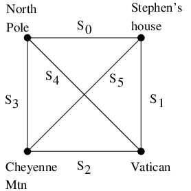
The lengths of the segments are:

Segment	Distance (km)	Cost ($)
S0: North Pole to Stephen's House	4,703km	$4.70
S1: Stephen's House to Vatican	9,074km	$9.09
S2: Vatican to Cheyenne Mtn	9,031km	$9.03
S3: Cheyenne Mtn to North Pole	5,696km	$5.70
S4: North Pole to Vatican	8,020km	$8.02
S5: Stephen's House to Cheyenne Mtn	1,709km	$1.71

We can now formulate a cost function to optimize. Let $x_j=1$ if segment $S_j$ appears in Santa's journey and $x_j =0$ otherwise. Then the total cost of the journey is: \begin{equation} C = \sum_{j=0}^5 C_j x_j \end{equation} where $C_0 = 4.70$, $C_1 = 9.09$, and so on. However, the problem also has constraints. Santa's journey must begin and end at the North Pole and he must visit each location exactly once. One can verify that out of all $2^6$ possible assignments to $x_0,\ldots,x_5$ only three are valid itineraries, namely:

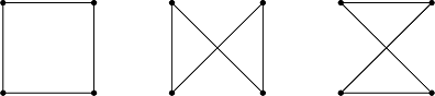
(It doesn't matter whether Santa goes clockwise or counterclockwise since the cost is the same.) One can further verify that the validity of the assignment to $x_0,\ldots,x_5 \in \{0,1\}$ is exactly captured by the following four constraints. \begin{equation} \sum_{j=0}^5 x_j = 4 \end{equation} \begin{equation} x_0 = x_2 \end{equation} \begin{equation} x_1 = x_3 \end{equation} \begin{equation} x_4 = x_5 \end{equation} Minimizing (1) subject to (2)-(5) is now a well formulated optimization problem. We can recast this as a problem of finding the ground state of a classical Ising model as follows. We work with variables \begin{equation*} z_0,\ldots,z_5 \in \{-1,1\} \end{equation*} and we map from $x_0,\ldots,x_5$ to $z_0,\ldots,z_5$ by: \begin{equation} z_j = 1 - 2 x_j \end{equation} i.e. if $x_j = 0$ then $z_j = 1$ and if $x_j = 1$ then $z_j = -1$. We thus wish to solve the following problem.

Problem 1: Find $z_0,\ldots,z_5 \in \{-1,1\}$ minimizing \begin{equation} C(z_0,\ldots,z_5) = \frac{1}{2} \sum_{j=0}^5 C_j (1-z_j) \end{equation} subject to: \begin{equation} \sum_{j=0}^5 z_j = -2 \end{equation} \begin{equation} z_0 = z_2 \end{equation} \begin{equation} z_1 = z_3 \end{equation} \begin{equation} z_4 = z_5 \end{equation}

To convert this into an unconstrained optimization problem we may add penalties to the cost function for violated constraints. One can see that \begin{equation} 1-z_i z_j = \left\{ \begin{array}{rl} 0 & \textrm{if $z_i = z_j$} \\ 2 & \textrm{if $z_i \neq z_j$} \end{array} \right. \end{equation} and \begin{equation} \left(2 + \sum_{j=0}^5 z_j \right)^2 = \left\{ \begin{array}{ll} 0 & \textrm{if $\sum_{j=0}^5 z_j = 2$} \\ \textrm{at least 2} & \textrm{otherwise} \end{array} \right. \end{equation} If we throw away all constraints then the minimum trip cost is zero (from $ x_0 = x_1 = x_2 = x_3 = x_4 = x_5 = 0$ ) and the maximum trip cost is $38.25 (from $x_0 = x_1 = x_2 = x_3 = x_4 = x_5 = 1 $ ). So, we see that if we choose a total cost function of: \begin{equation} H = \frac{1}{2} \sum_{j=0}^5 C_j (1 - z_j) + p (1-z_0 z_2) + p(1-z_1 z_3) + p (1-z_4 z_5) + p \left(2 + \sum_{j=0}^5 z_j \right)^2 \end{equation} then by choosing $ p > \frac{1}{2} 38.25 $ we ensure that all constraint-violating assignments are costlier than any valid assignment. For concreteness, we may choose $p = 20 $. Expanding (14) and using the fact that $z_j^2$ is always equal to 1 we arrive at classical Ising Hamiltonian whose ground state is the solution to the optimization problem.

Problem 2: Find $z_0,\ldots,z_5 \in \{-1,1\}$ minimizing \begin{equation} H_C = \sum_{i \lt j=0}^5 J_{ij} z_i z_j + \sum_{i=0}^5 h_i z_i \end{equation} where $h_j = 4p - \frac{1}{2} C_j$, $J_{02} = J_{13} = J_{45} = p$, and all other $ J_{i \lt j} = 2p $. Thus, with $p = 20$: \begin{eqnarray} h_0 & = & 77.65 \\ h_1 & = & 75.455 \\ h_2 & = & 75.485 \\ h_3 & = & 77.15 \\ h_4 & = & 75.99 \\ h_5 & = & 79.145 \\ \end{eqnarray} \begin{equation} J_{02} = J_{13} = J_{45} = 20 \end{equation} \begin{equation} J_{01} = J_{03} = J_{04} = J_{05} = J_{12} = J_{14} = J_{15} = J_{23} = J_{24} = J_{25} = J_{34} = J_{35} = 40 \end{equation}

Note that the minimum value achieved by $ H $ (i.e. the ground energy) is not the same as the minimum value achieved by C, because we have dropped the constant term from $ H $, keeping only terms that involve the variables $z_0,\ldots,z_5$. However, by construction, the assignment to the variables achieving this minimum will be the optimal solution to the original problem (problem 1).

2. Solving the Problem

Having formulated the problem, the next step is to solve it. One approach is to use the Quantum Approximate Optimization Algorithm (QAOA), introduced here. The idea behind QAOA (and quantum adiabatic optimization, which is closely related) is to first note that the classical Hamiltonian $H_C$ described in (15) can be promoted to a quantum Hamiltonian by replacing each variable $z_j$ with the Pauli-Z operator acting on the $j^{\mathrm{th}}$ qubit. (In keeping with the notation common in quantum information I'll denote this Pauli operator by $Z_j$. In other areas of physics it would be more common to denote this as $\sigma_z^{(j)}$.) We can thus solve our optimization problem by obtaining the ground state of the quantum Hamiltonian $H_C$ and then measuring the value of each qubit. In QAOA one attempts to do this by interspersing time evolutions according to the Hamiltonian $H_C$ with time evolutions induced by some "driver" Hamiltonian, which we will take to be \begin{equation} H_0 = -\sum_{i=0}^{n-1} X_i, \end{equation} where $ n$ is the number of qubits, in our case six. We initialize our system to the uniform superposition \begin{equation} \left( \frac{ | 0 \rangle + | 1 \rangle}{\sqrt{2}} \right)^{\otimes n} = \frac{1}{\sqrt{2^n}} \sum_{x \in \{0,1\}^n} | x \rangle, \end{equation} which, being a tensor product state, is easy to prepare.

We implement the unitary time evolutions $ e^{-i H_0 t}$ and $ e^{-i H_C t}$ as quantum circuits by breaking them down into elementary gates. Implementing $ e^{-i H_0 t} $ as a quantum circuit is not difficult because all the Pauli Pauli X operators commute, so \begin{equation} e^{-i H_0 t} = \prod_{j=0}^{n-1} e^{-i X_j t}. \end{equation} The Microsoft Quantum Development Kit (QDK) has gates of the form $ e^{-i X_j t/2} $ built in as R(PauliX, t, qubit[j]). Thus we can implement time evolution according to $ H_0 $ with the following Q# operation.

//This applies the X-rotation to each qubit. We can think of it as time evolution
//induced by applying H = - \Sum_i X_i for time t.
operation DriverHamiltonian(x: Qubit[], t: Double) : ()
{
    for(i in 0..Length(x)-1)
    {
        R(PauliX, -2.0*t, x[i]);
    }
}

Similarly, all the individual terms in $ H_C $ commute. These come in two types: single-qubit Pauli Z and two-qubit ZZ couplings. The single-qubit Z rotations can be implemented using R(PauliZ, t, qubit[j]), which is built in to the QDK. To implement the unitaries of the form $ e^{-i Z_i Z_j t}$ we note that this applies a phase determined by the exclusive-or of qubits i and j. Thus, we can compute this exclusive-or into an ancilla qubit, apply a Z-rotation on the ancilla, and then uncompute. Putting this all together (and cancelling some redundant CNOT gates) yields the following Q# function to implement $ e^{-i H_C t}$.

//This applies the Z-rotation according to the instance Hamiltonian. 
//We can think of it as Hamiltonian time evolution for time t induced
//by the Ising Hamiltonian \Sum_ij J_ij Z_i Z_j + \sum_i h_i Z_i.
operation InstanceHamiltonian(z: Qubit[], t: Double, h: Double[], J: Double[]) : Unit
{
    using (ancilla = Qubit[1])
    {
        for(i in 0..5)
        {
            R(PauliZ, 2.0*t*h[i],z[i]);
        }
        for(i in 0..5)
        {
            for (j in i+1..5)
            {
                CNOT(z[i], ancilla[0]);
                CNOT(z[j], ancilla[0]);
                R(PauliZ, 2.0*t*J[6*i+j], ancilla[0]);
                CNOT(z[i], ancilla[0]);
                CNOT(z[j], ancilla[0]);
            }
        }
    }
}

Then, we call these operations from an overall QAOA method as follows.

// Here is a QAOA algorithm for this Ising Hamiltonian
operation QAOA_santa(segmentCosts:Double[], penalty:Double, tx: Double[], tz: Double[], p: Int) : Bool[]
{
    // Calculate Hamiltonian parameters based on the given costs and penalty
    mutable J = new Double[36];
    mutable h = new Double[6];
    for (i in 0..5) {
        set h[i] = 4.0 * penalty - 0.5 * segmentCosts[i];
    }
    // Most elements of J_ij equal 2*penalty, so set all elements to this value, then overwrite the exceptions
    for (i in 0..35)
    {
        set J[i] = 2.0 * penalty;
    }
    set J[2]  = penalty;
    set J[9]  = penalty;
    set J[29] = penalty;
    // Now run the QAOA circuit
    mutable r = new Bool[6];
    using (x = Qubit[6])
    {
        ApplyToEach(H, x);                          // prepare the uniform distribution
        for (i in 0..p-1)
        {
            InstanceHamiltonian(x, tz[i], h, J);    // do Exp(-i H_C tz[i])
            DriverHamiltonian(x, tx[i]);            // do Exp(-i H_0 tx[i])
        }
        set r = MeasureAllReset(x);                 // measure in the computational basis
    }
    return r;
}

One of the key elements of a QAOA algorithm is a good choice of durations to apply the Hamiltonians. One good scheme, found through experimentation is to use five-round QAOA with the following parameters. \begin{equation} e^{-i H_0 t^{(x)}_4} e^{-i H_C t^{(z)}_4} \ldots e^{-i H_0 t^{(x)}_0} e^{-i H_C t^{(z)}_0} \left( \frac{|0\rangle + |1\rangle}{\sqrt{2}} \right)^{\otimes 6} \end{equation} where \begin{equation} t^{(x)}_0 = 0.619193 \quad t^{(x)}_1 = 0.742566 \quad t^{(x)}_2 = 0.060035 \quad t^{(x)}_3 = -1.568955 \quad t^{(x)}_4 = 0.045490 \end{equation} \begin{equation} t^{(z)}_0 = 3.182203 \quad t^{(z)}_1 = -1.139045 \quad t^{(z)}_2 = 0.221082 \quad t^{(z)}_3 = 0.537753 \quad t^{(z)}_4 = -0.417222 \end{equation} This succeeds in finding the optimal solution roughly 71% of the time. The full Q# code and C# driver implementing this is available on github. You are invited to download this code and try your own modifications. Perhaps you can find better parameters. Perhaps with enough help from your clever choices of parameters, and the power of quantum computing, Santa can conserve his budget enough to visit more than three destinations next year.